How to make your simulation study reproducible
eproducibility is crucial for simulation studies, not just for scientific transparency but also for debugging. When something goes wrong in your simulation, you need to be able to reproduce the exact same results to figure out what happened.
The Problem
Random number generation is, by definition, random. Each time you run your simulation, you get different results. This makes it impossible to debug issues or verify that changes to your code actually improve things.
# This gives different results each time
simple_simulation <- function() {
  x <- rnorm(100)
  y <- 2 * x + rnorm(100)
  lm(y ~ x)$coefficients[2]  # slope estimate
}

# Run it a few times
replicate(5, simple_simulation())
x x x x x
1.930130 1.973125 2.094085 2.152055 1.856361 The Solution: Seeds
The solution is to use set.seed() to make your random number generation reproducible:
# This gives the same result each time
reproducible_simulation <- function(seed = 123) {
  set.seed(seed)
  x <- rnorm(100)
  y <- 2 * x + rnorm(100)
  lm(y ~ x)$coefficients[2]
}

# Run it multiple times with the same seed
replicate(5, reproducible_simulation())
x x x x x
1.947528 1.947528 1.947528 1.947528 1.947528 # Different seeds give different results
map_dbl(1:5, reproducible_simulation)[1] 1.998940 1.952897 1.909835 1.851588 2.133111Simulation Study Framework
For a full simulation study, you need a more systematic approach. Here’s a framework that ensures reproducibility:
# Main simulation function
run_single_simulation <- function(n, effect_size, seed) {
  set.seed(seed)

  # Generate data
  x <- rnorm(n)
  y <- effect_size * x + rnorm(n)

  # Fit model
  model <- lm(y ~ x)

  # Extract results
  tibble(
    seed = seed,
    n = n,
    effect_size = effect_size,
    estimate = coef(model)[2],
    se = summary(model)$coefficients[2, 2],
    p_value = summary(model)$coefficients[2, 4]
  )
}

# Test it
run_single_simulation(n = 100, effect_size = 0.5, seed = 42)
# A tibble: 1 × 6
seed n effect_size estimate se p_value
<dbl> <dbl> <dbl> <dbl> <dbl> <dbl>
1 42 100 0.5 0.527 0.0877 0.0000000313Running Multiple Simulations
Now we can run many simulations with different seeds:
# Generate seeds for reproducibility
n_sims <- 1000
simulation_seeds <- sample.int(.Machine$integer.max, n_sims)

# Run the simulation study
simulation_results <- map_dfr(
  simulation_seeds,
  ~run_single_simulation(n = 100, effect_size = 0.5, seed = .x)
)

# Look at the results
head(simulation_results)
# A tibble: 6 × 6
seed n effect_size estimate se p_value
<int> <dbl> <dbl> <dbl> <dbl> <dbl>
1 97485668 100 0.5 0.574 0.109 0.000000829
2 561474357 100 0.5 0.399 0.116 0.000840
3 1628904358 100 0.5 0.440 0.101 0.0000325
4 2062762965 100 0.5 0.402 0.102 0.000156
5 361980619 100 0.5 0.346 0.0973 0.000571
6 536450273 100 0.5 0.469 0.0968 0.00000482 # Summary statistics
simulation_results %>%
summarise(
mean_estimate = mean(estimate),
sd_estimate = sd(estimate),
mean_se = mean(se),
coverage = mean(abs(estimate - 0.5) < 1.96 * se)
)# A tibble: 1 × 4
mean_estimate sd_estimate mean_se coverage
<dbl> <dbl> <dbl> <dbl>
1 0.502 0.103 0.101 0.946Visualizing Results
# Plot the distribution of estimates
p1 <- simulation_results %>%
  ggplot(aes(x = estimate)) +
  geom_histogram(bins = 50, alpha = 0.7) +
  geom_vline(xintercept = 0.5, color = "red", linetype = "dashed") +
  labs(title = "Distribution of Slope Estimates",
       subtitle = "Red line shows true value (0.5)",
       x = "Estimate", y = "Count")

# Plot estimates vs standard errors
p2 <- simulation_results %>%
  ggplot(aes(x = se, y = estimate)) +
  geom_point(alpha = 0.3) +
  geom_hline(yintercept = 0.5, color = "red", linetype = "dashed") +
  labs(title = "Estimates vs Standard Errors",
       x = "Standard Error", y = "Estimate")

# Combine plots
p1 / p2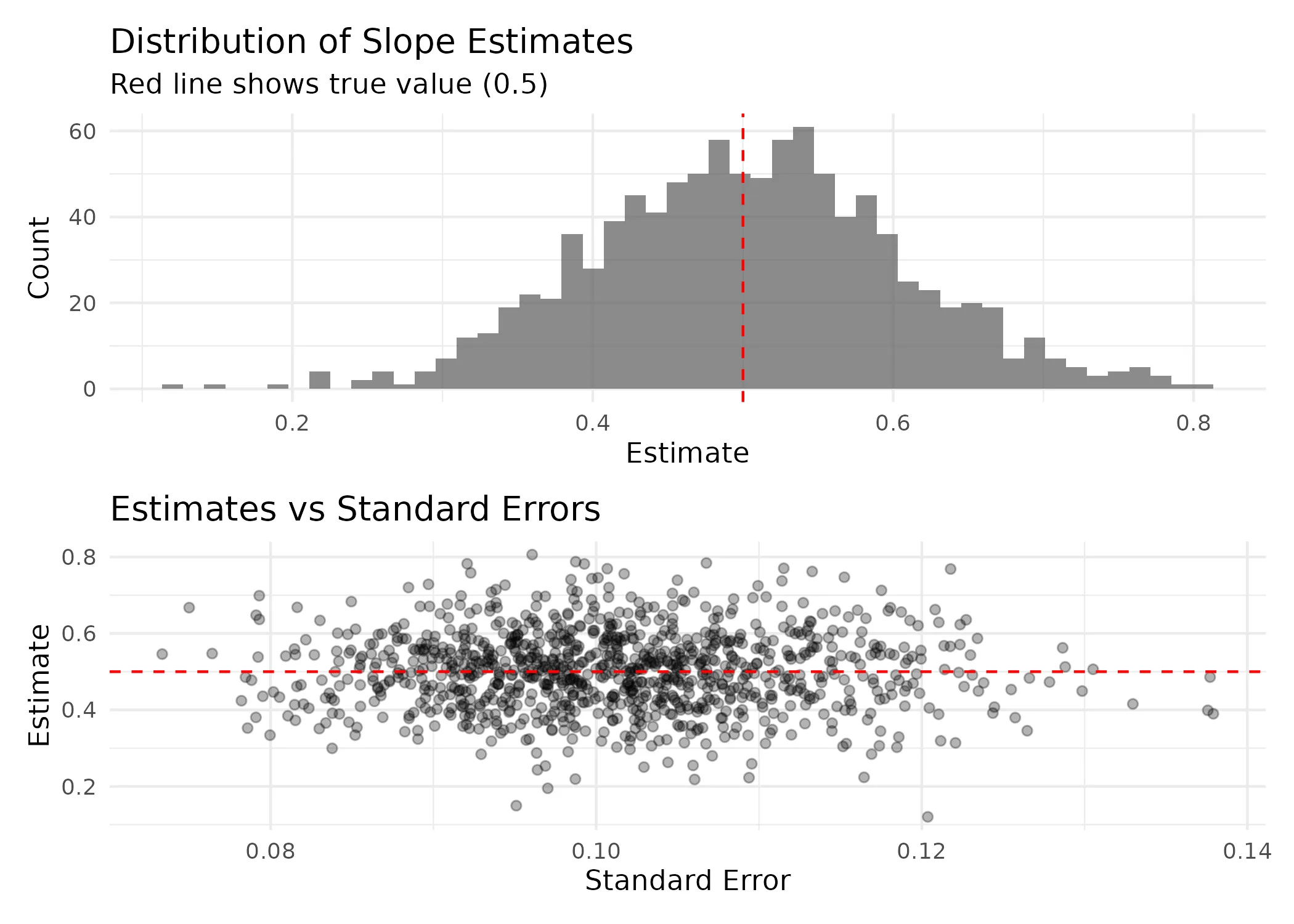
Advanced: Replicating Specific Results
Sometimes you want to reproduce just one specific simulation run that showed interesting behavior:
# Find simulations with unusually large estimates
outliers <- simulation_results %>%
  filter(abs(estimate - 0.5) > 0.2) %>%
  slice_head(n = 3)

print(outliers)
# A tibble: 3 × 6
seed n effect_size estimate se p_value
<int> <dbl> <dbl> <dbl> <dbl> <dbl>
1 323626374 100 0.5 0.746 0.100 3.75e-11
2 931722779 100 0.5 0.737 0.111 1.94e- 9
3 1222203724 100 0.5 0.708 0.0936 2.10e-11# Replicate these specific results
replicated_outliers <- map_dfr(
outliers$seed,
~run_single_simulation(n = 100, effect_size = 0.5, seed = .x)
)
# Check they match exactly
all.equal(outliers, replicated_outliers)[1] TRUEParallel Processing with Seeds
When using parallel processing, you need to be careful about seed management:
# Set up parallel processing
plan(multisession, workers = 2)

# This version works with parallel processing
run_simulation_parallel <- function(seeds, n, effect_size) {
  future_map_dfr(
    seeds,
    ~run_single_simulation(n = n, effect_size = effect_size, seed = .x),
    .options = furrr_options(seed = TRUE)
  )
}

# Run a smaller simulation in parallel
parallel_seeds <- sample.int(.Machine$integer.max, 100)
parallel_results <- run_simulation_parallel(
  seeds = parallel_seeds,
  n = 100,
  effect_size = 0.5
)

# Clean up
plan(sequential)

head(parallel_results)
# A tibble: 6 × 6
seed n effect_size estimate se p_value
<int> <dbl> <dbl> <dbl> <dbl> <dbl>
1 1072799182 100 0.5 0.454 0.0829 0.000000336
2 1883428151 100 0.5 0.484 0.0902 0.000000530
3 691665735 100 0.5 0.494 0.0879 0.000000176
4 883159953 100 0.5 0.511 0.0971 0.000000846
5 1332206612 100 0.5 0.632 0.110 0.000000101
6 1578395705 100 0.5 0.518 0.104 0.00000261 Best Practices
- Always set seeds: Every simulation should have a seed parameter
- Use different seeds for different runs: Don’t reuse the same seed
- Save your seeds: Store them so you can replicate specific results
- Document your RNG: Note which version of R and packages you used
- Test reproducibility: Verify that re-running gives identical results
# Example of a well-structured simulation function
well_structured_simulation <- function(
  n_sims = 1000,
  n = 100,
  effect_size = 0.5,
  base_seed = 42
) {
  # Generate reproducible seeds
  set.seed(base_seed)
  sim_seeds <- sample.int(.Machine$integer.max, n_sims)

  # Store metadata
  metadata <- list(
    n_sims = n_sims,
    n = n,
    effect_size = effect_size,
    base_seed = base_seed,
    r_version = R.version.string,
    date = Sys.time()
  )

  # Run simulations
  results <- map_dfr(
    sim_seeds,
    ~run_single_simulation(n = n, effect_size = effect_size, seed = .x)
  )

  # Return both results and metadata
  list(
    results = results,
    metadata = metadata,
    seeds = sim_seeds
  )
}

# Run the simulation
final_simulation <- well_structured_simulation()

# Check reproducibility
final_simulation_2 <- well_structured_simulation()
identical(final_simulation$results, final_simulation_2$results)
[1] TRUEConclusion
Reproducible simulation studies are essential for:
- Debugging: Finding and fixing problems in your code
- Verification: Ensuring changes actually improve results
- Transparency: Allowing others to verify your findings
- Efficiency: Not having to re-run everything when you find a bug
The key principles are:
- Use seeds consistently
- Save your seeds and metadata
- Test that your code actually reproduces results
- Document your computational environment
Remember: “Replication is not only important for science but also for debugging, which in turn is elementary to science.”
References
- R Core Team (2022). R: A language and environment for statistical computing. R Foundation for Statistical Computing, Vienna, Austria.
- Wickham, H. (2019). Advanced R, Second Edition. Chapman and Hall/CRC.